
No New Year without its New Year resolution. So how about diving into computer vision, learning a new library that allows you to train a computer vision model in less than 30 lines of code and revisiting some good old fairy tales? And all at once?
Hans Christian Andersen’s tale of the ugly duckling tells us about a cygnet (i.e. a baby swan) brought up as part of a family of ducks and being bullied by its siblings and everybody else for being ugly (read different to them). If only the poor cygnet had had somebody to tell it that it in fact was a swan instead! Entering Our Hero, Machine Learning to the rescue!
In this project, we will learn how to use fastai, Gradio and HuggingFace to build a magic mirror that can distinguish a duckling from a cygnet in four main steps. Then we will deploy it to the internet for all ducklings out there to use. We will learn how to:
- Create a dataset from scratch, using a duckduckgo image search.
- Train a train a computer vision model using fastai.
- Build a magic mirror app using Gradio.
- Deploy the magic mirror for free on Hugging Face.
If you want to follow along, you can find the complete code in the GitHub repository Tales-of-1001-Data. If you want to try out the app, find it deployed on my ugly-duckling-magic-mirror Hugging Face space.
So let’s get started to help the duckling answer the magical question…

Mirror, mirror on the wall, am I a duckling or a cygnet after all?
Preparations
Installing Libraries
The training part of this notebook requires two non-standard libraries:
- We use
duckduckgo_searchto search for cygnet and duckling images to create the dataset. - We use
fastaifor training the computer vision model. fastai. Fastai is a higher-level interface to PyTorch that allows users to train to train deep learning models in very few lines of code (here is an example of four lines of code from zero to image-classifier).
If you run your code on Google Colab (because yeah, free GPUs!), you don’t need need to worry about installing fastai, just run ! pip install duckduck-go to install the duckduck-go library. Anywhere else, you might have to install fastai, too. At the time of writing, the fastai homepage recommends mamba for installation, but it’s worth checking again.
Importing Modules
Library imports should happen at the top of your code, so let’s import the required libraries.
from pathlib import Path
from time import sleep
from dataclasses import dataclass
from typing import List

from duckduckgo_search import ddg_images

from fastai.data.transforms import get_image_files, parent_label, RandomSplitter

from fastai.interpret import ClassificationInterpretation

from fastai.metrics import error_rate

from fastai.vision.augment import Resize, RandomResizedCrop, aug_transforms
from fastai.vision.core import DataBlock
from fastai.vision.data import CategoryBlock, ImageBlock
from fastai.vision.all import vision_learner # import from vision.all due to patching
from fastai.vision.utils import download_images, get_image_files, verify_images

from fastcore.foundation import L

from torchvision.models.resnet import resnet18
Note that due to the large number of required imports and the extensive monkey patching in the library the recommended way of importing fastai libraries is to use from fastai import * or from fastai.vision.all import * (take a look at walk-with-fastai’s first lesson to get an impression of the extend of both).
However, since wildcard imports are typically discouraged (with exceptions for ad-hoc work), I tend to import the libraries one by one and resolve issues as they appear. This also forces me to become more familiar with the internal organization of the library itself, something I appreciate. When running into issues I find the following steps helpful.
How to troubleshoot imports
- Run
from fastai import *to see if this solves your issue. - If so, use
which functionnameto find out from where you should be actually importing your library - Adapt your import statement accordingly.
An example of one of these patching issues is that vision_learner should be imported from fastai.vision.all instead of from fastai.vision.learner.
If you in general don’t want to go into too many details with your imports, you can also strike a happy medium by importing modules from fastai.vision.all.
Creating the Dataset
No machine learning without data. To create our dataset, we implement the following steps:
- Use duckduckgo’s image search to get a list of urls of images of ducklings and cygnets.
- Download the images to our system using fastai’s
download_images(). - Check if the downloaded images are ok using fastai’s
verify_images(). - Delete images which are not ok.
Once we have built the dataset, we will use it to train a classifier. A common image classification folder structure is to save the images in folders named according to their label. To decouple the label from the actual search term and create more flexibility in setting up our search, we create a Searchterm dataclass that holds both the search term and the label.
IMAGEPATH = Path().cwd()/'images'

@dataclass
class Searchterm:
  searchstring: str
  label: str


def search_images(searchterm: str, max_results: int) -> L:
    """Uses duckduckgo to search for images"""

    return L(ddg_images(searchstring,
                        max_results=max_results)).itemgot('image')


def delete_invalid_images(imagepath: Path) -> int:
    """Deletes invalid images in imagepath"""

    invalid_images = verify_images(get_image_files(imagepath))
    invalid_images.map(Path.unlink)
    return len(invalid_images)


def download_search_data(terms: List[Searchterm], n_searches) -> None:
    """Searches for images and downloads results"""
    for term in terms:
        print(f"Downloading {n_searches} images for {term.searchstring} into folder {term.label}.")
        folder = IMAGEPATH/term.label
        folder.mkdir(parents=True, exist_ok=False)

        download_images(folder,
                        urls=search_images(f"{term.searchstring}",
                                        max_results=n_searches))

        print(f"Deleted {delete_invalid_images(IMAGEPATH/term.label)} invalid images for {term.searchstring}")
On Finding the Right Search Terms
To make sure that one downloads a useful dataset, it helps to start the process by manually running a few searches and having a look at the general results of the query. Doing this process manually allows you to quickly tweak your query string till it returns useful images and helps to avoid the garbage in - garbage out problem.
For this project, I found that searching for “cygnet” not only returned images of actual cygnets, but also returned images wool and alcohol bottles (both of brands with “cygnet” in the name). There are technical ways of dealing with this problem, but the most straight forward solution is to simply change the search string to “baby swan”, which solved the issue perfectly. In a similar project, I wanted to get photos in different lighting conditions, but realized that whilst looking for “objectname sun” returned useful results, looking for “objectname shade” did mostly return undesired results, so was not recommendable.
Once we have found good search strings, we can run our search and download some images! The following code downloads 100 images for “baby swan” and “duckling” each, checks them and deletes broken images. In my experience, about 2-3 images are typically broken, so afterwards we are left with a little under 100 actual images.
# Clean folder structure to avoid imbalanced data sets
IMAGEPATH.delete()

download_search_data([Searchterm(searchstring='baby swan', label='cygnet'),
                      Searchterm(searchstring='duckling', label='duckling')],
                     n_searches=100)
Training the Image Classifier
Setting up the DataLoader
Next, we need to tell fastai how to convert the images in their folders into image batches that it can train the classifier on. fastai loads data using a Dataloaders object, so we need to tell it how to create one. One way to create a DataLoaders object is to first create a DataBlock, then call the dataloaders() method on it. The five things we need to tell fastai when creating a DataLoaders object are:
- What type of data are input and output data?
- How should it load the data?
- For a classification task: How can it determine the labels?
- How should it create a validation set?
- Which data transformations should it apply? Are these individual or batch transformations?
Data Transformations: Image Resizing and Augmentation
Data transformations come in two flavours, individual and batch transformations. Individual transformations are applied to each image individually, batch transformations are applied to a whole batch in parallel at the same time (making them a lot faster).
Typical data transformations for image data are resizing and image augmentation tasks. In order to train a neural network on image data, the images need to be of the same size. We can achieve this through:
- cropping
- squishing
- padding
All of these have their drawbacks. Cropping might delete important parts of the image, squishing distorts the image and padding introduces useless data points thereby unnecessarily increasing computational costs.
In order to prevent over-fitting (especially when dealing with small datasets), we might also apply augmentations to our image dataset. Augmentations can happen on an image or on a pixel level. Examples of augmentations on an image level are:
- flipping
- rotation
- perspective warping
Examples of pixel augmentations are changes to:
- brightness
- saturation
- hue
- contrast
Different augmentations are applied in each batch.
Here is how this can look like for our example:
birds = DataBlock(blocks=(ImageBlock, CategoryBlock),
                  get_items=get_image_files,
                  get_y=parent_label,
                  splitter=RandomSplitter(valid_pct=0.2, seed=42),
                  item_tfms=[RandomResizedCrop(256, min_scale=0.8)],
                  batch_tfms=aug_transforms())

dls = birds.dataloaders(IMAGEPATH, bs=64)
Let’s look at the inputs to DataBlock in more detail.
-
blocks=(ImageBlock, CategoryBlock)Trains an image classifier: images as input, categories as output.
-
get_items=get_image_filesLoads the images by applying the
get_image_filesfunction to the path specified as input to thedataloadersfunction. -
get_y=parent_labelGets the image labels by using the
parent_labelfunction, which extracts the label from the folder name. -
splitter=RandomSplitter(valid_pct=0.2, seed=42)Splits the data into training and validation sets by randomly assigning 20% of the data to the validation set. Seeds the random number generator to 42. Note that
Dataloadersforces you to adhere to best practice and create a validation set. Here, we seed the random number generator to make the split reproducible across multiple runs. As always it’s completely up to you which seed you choose (even though 42 is often used). -
item_tfms=[RandomResizedCrop(256, min_scale=0.8)]Applies the item transformation
RandomResizedCrop(). Randomly crops a part of the image (keeping at least 80% of the original image), then scales it to 256x256 pixels. A different random crop is selected for each batch. -
batch_tfms=aug_transforms()Applies the batch transformation
aug_transforms(), which is a set of transformations designed by fastai to work well for natural photos.
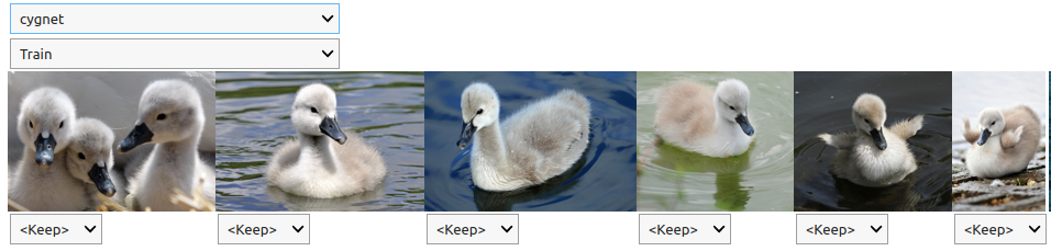
Having created our data set batches, let’s inspect a few of the resulting images (including their augmentations).
# Inspect some images
dls.train.show_batch(max_n=6, nrows=1)
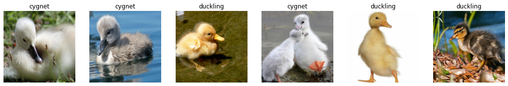
Looking good :) Next, we set up the learning part.
Setting up the Learner
We use fastai’s vision_learner() function to create a Residual Neural Network (ResNet) with 18 hidden layers. ResNets counteract the problem of vanishing gradients by including skip-layers in their architecture. Skip-layers allow gradient information to propagate through the network more easily by adding the output of previous layers to layers deeper in the network. This allows for the training of deeper networks (the original paper demonstrated the successful training of a 152-layer network and even experimented with up to 1002 layers). The ResNet-18 architecture is the smallest ResNet architecture, making it quite fast to train. Whilst smaller networks can result in lower prediction accuracy, a ResNet-18 archicture is perfectly suitable for our toy problem.
In order to achieve good results with few training iterations and a small dataset, we take advantage of transfer learning. In transfer learning, we initialize the model weights with weights that have been trained on a large corpus of data and fine-tune only some of them to our specific problem (often we might change only the weights of the actual classification layer). By default, fastai uses weights which were pre-trained using the ImageNet corpus.
To find a good number of fine-tuning steps (good accuracy without overfitting), we train the model while we observe training and validation losses. While the training loss will continue to go down with more training steps, the validation loss will first decrease, then eventually start increasing again when the model starts overfitting to the training data. This point of onsetting overfitting gives as a good number of training steps. In our case, this is about 5.
Let’s train the model!
learn = vision_learner(dls, resnet18, metrics=error_rate)
learn.fine_tune(5)
| epoch | train_loss | valid_loss | error_rate | time |
|---|---|---|---|---|
| 0 | 1.322290 | 0.665758 | 0.243243 | 00:56 |
| epoch | train_loss | valid_loss | error_rate | time |
|---|---|---|---|---|
| 0 | 0.537393 | 0.333642 | 0.135135 | 00:58 |
| 1 | 0.390109 | 0.203725 | 0.081081 | 00:58 |
| 2 | 0.283819 | 0.161411 | 0.054054 | 00:58 |
| 3 | 0.218951 | 0.160250 | 0.054054 | 01:00 |
| 4 | 0.174419 | 0.154186 | 0.054054 | 00:57 |
Evaluating Your Model
Having trained the model, let’s evaluate its performance. Whilst loss is the algorithm’s metric of driving the optimization to better results, it’s not a very humanly understandable metric. So let’s look at the confusion matrix instead to see how well our model is performing.
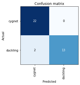
Confusion Matrix
The confusion matrix compares the predicted with the true class for each image and shows us a summary for all images in the validation set. Below, we see that all cygnets in the validation set were correctly classified as such, whilst two of the ducklings were misclassified as cygnets. Overall not too bad an outcome.
interp = ClassificationInterpretation.from_learner(learn)
interp.plot_confusion_matrix()
Largest Losses
For a more detailed view, let’s go back to the losses. Using interp.plot_top_losses(), we can display the images with the highest losses. A higher loss means that either the algorithm has correctly predicted the class of an image, but is not very certain of it or it has incorrectly predicted the class of an image (the more certain of an incorrect prediction it is, the higher is the loss).
interp.plot_top_losses(10, nrows=2)
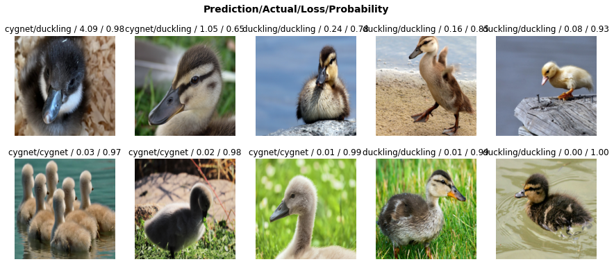
The two largest contributions to the loss are the two misclassified ducklings, which we have already encountered in teh classification matrix, followed by correctly classified images, but with less certainty. We see that image with the largest loss is an image of a duckling that looks very different from most of the other ducklings in the dataset. Without being a ornithologist, my impression is that most of the ducklings in the dataset are Mallard ducklings, whilst this one might not be. Unfortunately I could not find which type of duck this might be (any ornithologist willing to help?). This is a good demonstration that it is always worth to keep track of where your data is coming from (in this case URLs, image captions, etc). It makes these type of investigations a lot easier. Going back to the original task, if we were serious about good performance, it might be beneficial to deal with these dataset outliers by for example eliminating everything which isn’t a Mallard duckling from our dataset (assuming that our users are only interested in classifying Mallards that is) or adding more ducklings of other types to the data.
To find the associated files to your losses, use interp.top_losses(items=True) to display all losses together with the associated file paths.
More Data Cleaning Options
Another handy tool for image data cleaning is the ImageClassifierCleaner() function. Apply it to a learner to get a drop-down interface allowing you to easily relabel or delete images from your dataset.
from fastai.vision.widgets import ImageClassifierCleaner

cleaner = ImageClassifierCleaner(learn)
cleaner
Note that this only provides the graphical interface, you still need to perform the actual relabelling/deleting. You can do this by using the following code. Run it for each combination of drop-downs that you want to treat.
import shutil

def execute_cleaning(cleaner):
    """Applies deletion/renaming operations to files"""

    for idx in cleaner.delete():
       cleaner.fns[idx].unlink()

    for idx, category in cleaner.change():
       shutil.move(str(cleaner.fnx[idx], IMAGEPATH/category))
Exporting the Model
Finally we export the model for later use. In the next step, we will see how to export it to Hugging Face to deploy it.
learn.export('duckling_learner.pkl')
Building a Gradio Interface on HuggingFace
Now that we have a trained model, we want to wrap it in a user interface and host it to share it with all the cygnets and ugly ducklings out there. Luckily, there are plenty of options to host ML based apps for free. Where you can do so, will also depend on how you decide to implement the interface.
Some easy, straight-forward, python based options for building graphical model interfaces are:
- Gradio
- Streamlit
- Voila
Depending on your choice of GUI, some options to serve your interface are:
- Gradio: Hugging Face
- Streamlit: Hugging Face, Streamlit Community
- Voila: GitHub, Binder
Here, I will show how to build an app using Gradio and host it on Hugging Face. This is mostly because I had used some of the other ones in the past and wanted to try out something new. Either of the options above will serve you well.
This is how my Gradio app looks like. To try it out for yourself, find its live version on HuggingFace.
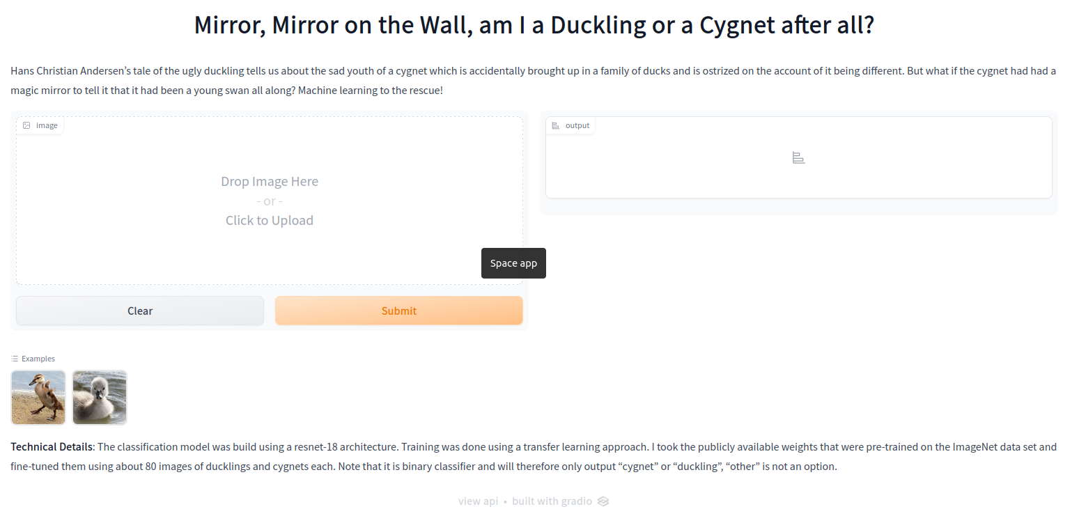
In order to host a Gradio app like the one shown above on Hugging Face, you need six files:
- the main file defining the Gradio app
- the ML model for scoring
- a
README.mddefining the app’s metadata (eg its title) - a
requirements.txtfile defining extra packages that need to be installed - a
.gitignorefile (telling Hugging Face’s git which files to ignore and which to handle usinggit-lfs) - (optional) the example images that the user can click on
Let’s go through the files one-by-one. If you want to check out the exact files, you can find them in my ugly-duckling Hugging Face space.
File 1: Main File - Gradio App
This is the complete code for the Gradio interface (with texts abbreviated for shortness):
from pathlib import Path
from fastai.vision.learner import load_learner
import gradio as gr

MODELPATH='cygnet-vs-duckling.pkl'

LEARN = load_learner(MODELPATH)

def classify_image(image):
    _, _, probs = LEARN.predict(image)
    return dict(zip(LEARN.dls.vocab, map(float, probs)))

title = 'Mirror, Mirror on the Wall, am I a Duckling or a Cygnet after all?'
description = """Hans Christian Andersen's tale of ..."""

examples = ['duckling.jpg', 'cygnet.jpg']

article = '**Technical Details**: The classification model was build using ...'

app = gr.Interface(fn=classify_image,
                   inputs=gr.components.Image(),
                   outputs=gr.components.Label(),
                   examples=examples,
                   title=title,
                   description=description,
                   article=article,
                   allow_flagging='never')

app.launch()
Easy, right? But what does it do? Let’s start by looking at the Interface function.
The parameters of the Interface function tell Gradio that it should take an image as an input and generate a label as output using the scoring function classify_image. Gradio expects the scoring function to output a dictionary with the labels as keys and the associated probabilities as values. Note that predict returns the probabilities as tensors, which means that we need to convert them to floats for Gradio to be able to handle.
File 2: ML Model
We need to upload the previously saved model to Hugging Face so that we can use it for scoring. In order to be able to upload the model, you need to have Git-LFS installed and enabled in your repository. Git-LFS (Large File Storage) is a Git extension that allows you to download large files in your repository lazily, which makes them easier to handle and reduces your repository size.
File 3: Metadata - Readme.md
The Readme.md contains the metadata for the app. For the full details, see the ugly ducklings Readme on Hugging Face.
File 4: Dependencies - Requirements.txt
Since we have already told Hugging Face to use Gradio in the Readme, gradio get automatically installed in the workspace. So the only external library to install is fastai, leaving the requirements file with a single line, reading fastai.
File 5: Handling Files in Git: .gitignore
The .gitignore file comes with the HuggingFace repository. You can use it as it is.
File(s) 6 (optional): Example Images
If you have specified example images, you need to upload them. Again, Git-LFS is required.
And that’s it! Upload everything to Hugging Face and tell your friends! :)
Final Thoughts
The model produced here is a toy model to demonstrate the overall workflow with many short-comings. One of them is that it is a binary classifier, where the categories do not span the entire possible space. This means that the classifier has to decide if it thinks that the image is more likely a duckling or more likely a cygnet. Saying “Don’t be silly, this image is clearly a pineapple!” is just not an option. With that being said, I will leave you to marvel (or maybe chuckle?) at the following…
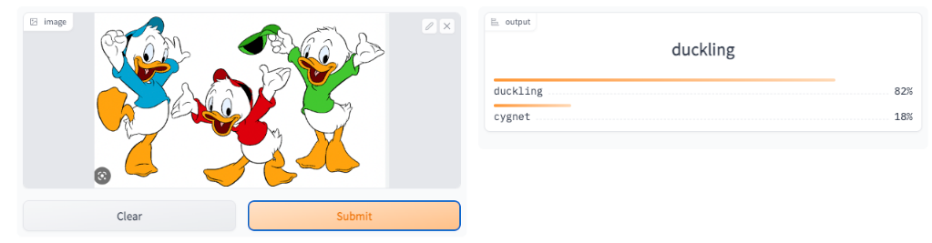
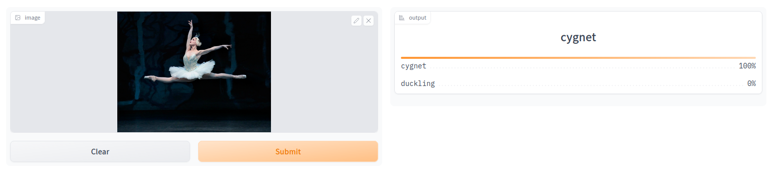
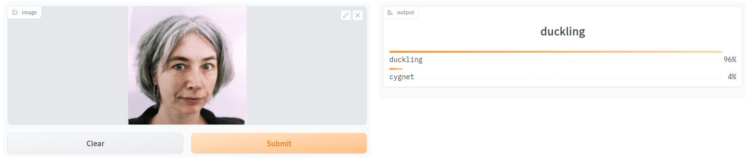
And finally, I tried it out on myself… Apparently I am more of a duckling than Huey, Dewey and Louie together. Not sure what my self-esteem has to say to that …
Leave a Comment