
Note: Pandas version 0.20.1 (May 2017) changed the grouping API. This post reflects the functionality of the updated version.
Anyone working with data knows that real-world data is often patchy and cleaning it takes up a considerable amount of your time (80/20 rule anyone?). Having recently moved from Pandas to Pyspark, I was used to the conveniences that Pandas offers and that Pyspark sometimes lacks due to its distributed nature. One of the features I have learned to particularly appreciate is the straight-forward way of interpolating (or in-filling) time series data, which Pandas provides. This post is meant to demonstrate this capability in a straight forward and easily understandable way using the example of sensor read data collected in a set of houses. It will be followed up with a second post about how to achieve the same functionality in PySpark. The full notebook for this post can be found here in my github.
Preparing the Data and Initial Visualization
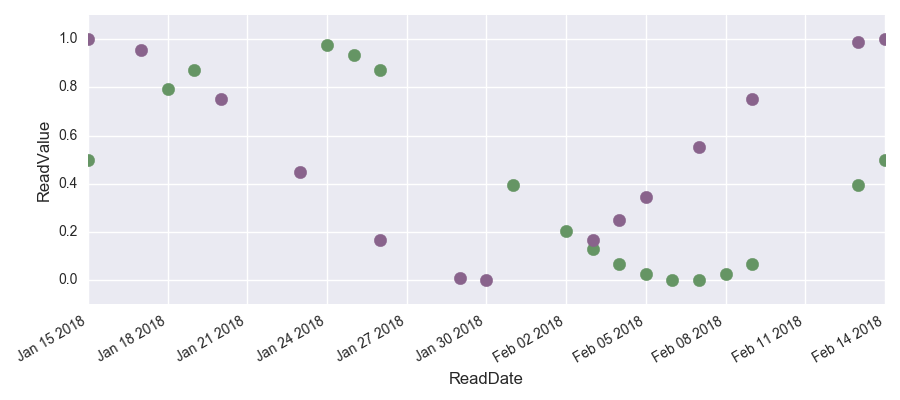
First we generate a pandas data frame df0 with some test data. We create a data set containing two houses and use a \(sin\) and a \(cos\) function to generate some read data for a set of dates. To generate the missing values, we randomly drop half of the entries.
data = {'datetime': pd.date_range(start='1/15/2018', end='02/14/2018', freq='D')\
                .append(pd.date_range(start='1/15/2018', end='02/14/2018', freq='D')),
        'house' : ['house1' for i in range(31)] + ['house2' for i in range(31)],
        'readvalue':  [0.5 + 0.5*np.sin(2*np.pi/30*i) for i in range(31)]\
                    + [0.5 + 0.5*np.cos(2*np.pi/30*i) for i in range(31)]}
df0 = pd.DataFrame(data, columns = ['datetime', 'house', 'readvalue'])

# Randomly drop half the reads
random.seed(42)
df0 = df0.drop(random.sample(range(df0.shape[0]), k=int(df0.shape[0]/2)))
This is how the data looks like. A \(sin\) and a \(cos\) with plenty of missing data points.
We will now look at three different methods of interpolating the missing read values: forward-filling, backward-filling and interpolating. Remember that it is crucial to choose the adequate interpolation method for the task at hand. Special care needs to be taken when looking at forecasting tasks (for example if you want to use your interpolated data for forecasting weather than you need to remember that you cannot interpolate the weather of today using the weather of tomorrow since it is still unknown).
In order to interpolate the data, we will make use of the groupby() function followed by resample(). However, first we need to convert the read dates to datetime format and set them as index of our dataframe:
df = df0.copy()
df['datetime'] = pd.to_datetime(df['datetime'])
df.index = df['datetime']
del df['datetime']
This is how the structure of the dataframe looks like now:
df.head(1)
| house | readvalue | |
|---|---|---|
| datetime | ||
| 2018-01-15 | house1 | 0.5 |
Interpolation
Since we want to interpolate for each house separately, we need to group our data by ‘house’ before we can use the resample() function with the option ‘D’ to resample the data to daily frequency.
The next step is then to use mean-filling, forward-filling or backward-filling to determine how the newly generated grid is supposed to be filled.
mean()
Since we are strictly upsampling, using the mean() method, all missing read values are filled with NaNs:
df.groupby('house').resample('D').mean().head(4)
| readvalue | ||
|---|---|---|
| house | datetime | |
| house1 | 2018-01-15 | 0.500000 |
| 2018-01-16 | NaN | |
| 2018-01-17 | NaN | |
| 2018-01-18 | 0.793893 |
pad() - forward filling
Using pad() instead of mean() forward-fills the NaNs.
df_pad = df.groupby('house')\
            .resample('D')\
            .pad()\
            .drop('house', axis=1)
df_pad.head(4)
| readvalue | ||
|---|---|---|
| house | datetime | |
| house1 | 2018-01-15 | 0.500000 |
| 2018-01-16 | 0.500000 | |
| 2018-01-17 | 0.500000 | |
| 2018-01-18 | 0.793893 |
bfill - backward filling
Using bfill() instead of mean() backward-fills the NaNs:
df_bfill = df.groupby('house')\
            .resample('D')\
            .bfill()\
            .drop('house', axis=1)
df_bfill.head(4)
| readvalue | ||
|---|---|---|
| house | datetime | |
| house1 | 2018-01-15 | 0.500000 |
| 2018-01-16 | 0.793893 | |
| 2018-01-17 | 0.793893 | |
| 2018-01-18 | 0.793893 |
interpolate() - interpolating
If we want to mean interpolate the missing values, we need to do this in two steps. First, we generate the data grid by using mean() to generate NaNs. Afterwards we fill the NaNs by interpolated values by calling the interpolate() method on the readvalue column:
df_interpol = df.groupby('house')\
                .resample('D')\
                .mean()
df_interpol['readvalue'] = df_interpol['readvalue'].interpolate()
df_interpol.head(4)
| readvalue | ||
|---|---|---|
| house | datetime | |
| house1 | 2018-01-15 | 0.500000 |
| 2018-01-16 | 0.597964 | |
| 2018-01-17 | 0.695928 | |
| 2018-01-18 | 0.793893 |
Visualizing the Results
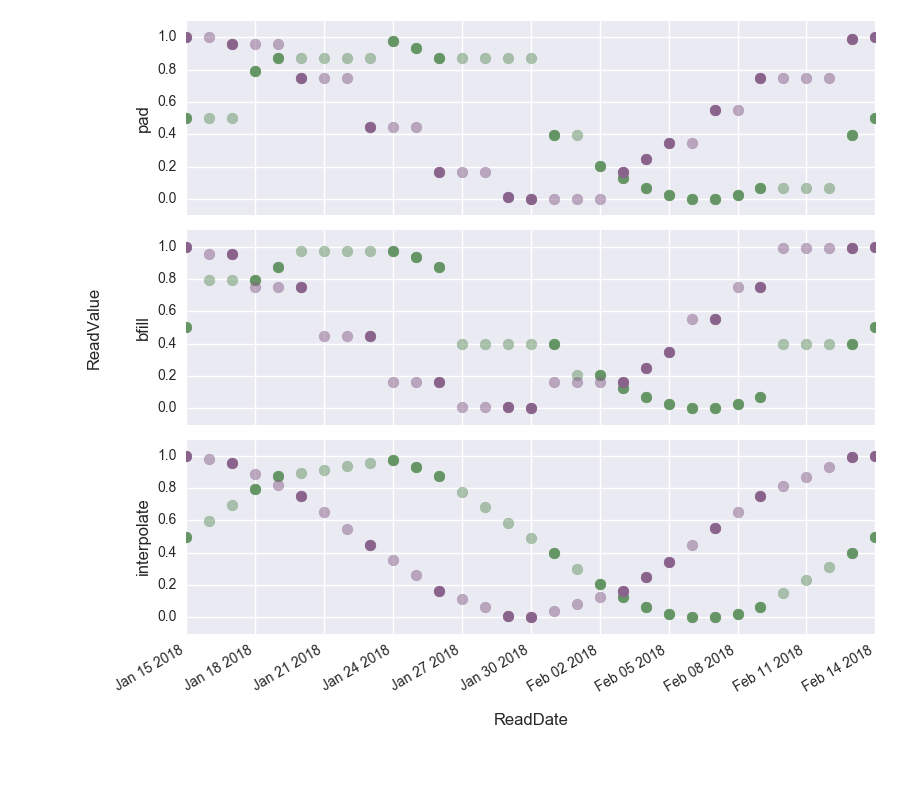
Finally we can visualize the three different filling methods to get a better idea of their results. The opaque dots show the interpolated values.
We can clearly see how in the top figure, the gaps have been filled with the last known value, in the middle figure, the gaps have been filled with the next value to come and in the bottom figure the difference has been interpolated.
Summary
In this blog post we have seen how we can use Python Pandas to interpolate time series data using either backfill, forward fill or interpolation methods. Having used this example to set the scene, in the next post, we will see how to achieve the same thing using PySpark.
Leave a Comment