
Anyone working with data knows that real-world data is often patchy and cleaning it takes up a considerable amount of your time (80/20 rule anyone?). Having recently moved from Pandas to Pyspark, I was used to the conveniences that Pandas offers and that Pyspark sometimes lacks due to its distributed nature. One of the features I have been particularly missing recently is a straight-forward way of interpolating (or in-filling) time series data. Whilst the problem of in-filling missing values has been covered a few times (e.g. here), I was not able to find a source, which detailed the end-to-end process of generating the underlying time-grid and then subsequently filling in the missing values. This post tries to close this gap. Starting from a time-series with missing entries, I will show how we can leverage PySpark to first generate the missing time-stamps and then fill-in the missing values using three different interpolation methods (forward filling, backward filling and interpolation). This is demonstrated using the example of sensor read data collected in a set of houses. Note that this post follows closely the structure of last week’s post, where I demonstrated how to do the end-to-end procedure in Pandas. The full code for this post can be found here in my github.
Preparing the Data and Visualization of the Problem
In order to demonstrate the procedure, first, we generate some test data. The data set contains data for two houses and uses a \(sin()\) and a \(cos()\) function to generate some sensor read data for a set of dates. To generate the missing values, we randomly drop half of the entries.
import pandas as pd
import numpy as np
import random
data = {'readtime': pd.date_range(start='1/15/2018', end='02/14/2018', freq='D')\
                .append(pd.date_range(start='1/15/2018', end='02/14/2018', freq='D')),
        'house' : ['house1' for i in range(31)] + ['house2' for i in range(31)],
        'readvalue': [0.5+0.5*np.sin(2*np.pi/30*i) for i in range(31)]\
                + [0.5+0.5*np.cos(2*np.pi/30*i) for i in range(31)]}
df0 = pd.DataFrame(data, columns = ['readtime', 'house', 'readvalue'])

random.seed(42)
df0 = df0.drop(random.sample(range(df0.shape[0]), k=int(df0.shape[0]/2)))
df0.head()
| readtime | house | readvalue | |
|---|---|---|---|
| 0 | 2018-01-15 | house1 | 0.500000 |
| 3 | 2018-01-18 | house1 | 0.793893 |
| 4 | 2018-01-19 | house1 | 0.871572 |
| 9 | 2018-01-24 | house1 | 0.975528 |
| 10 | 2018-01-25 | house1 | 0.933013 |
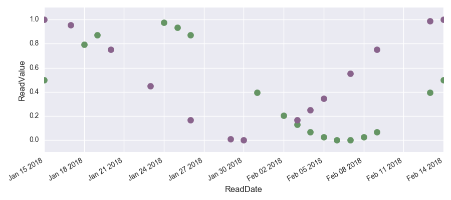
The following graph shows the data with the missing values clearly visible.
To parallelize the data set, we convert the Pandas data frame into a Spark data frame. Note, that we need to divide the datetime by 10^9 since the unit of time is different for pandas datetime and spark. We also add the column ‘readtime_existent’ to keep track of which values are missing and which are not.
import pyspark.sql.functions as func
from pyspark.sql.functions import col

df = spark.createDataFrame(df0)
df = df.withColumn("readtime", col('readtime')/1e9)\
        .withColumn("readtime_existent", col("readtime"))
We get a table like this:
| readtime | house | readvalue | readtime_existent |
|---|---|---|---|
| 1.5159744E9 | house1 | 0.500000 | 1.5159744E9 |
| 1.5162336E9 | house1 | 0.793893 | 1.5162336E9 |
| 1.51632E9 | house1 | 0.871572 | 1.51632E9 |
Interpolation
Resampling the Read Datetime
The first step is to resample the time data. If we were working with Pandas, this would be straight forward, we would just use the resample() method. However, Spark works on distributed datasets and therefore does not provide an equivalent method. Obtaining the same functionality in PySpark requires a three-step process. In the first step, we group the data by house and generate an array containing an equally spaced time grid for each house. In the second step, we create one row for each element of the arrays by using the spark sql function explode(). In the third step, the resulting structure is used as a basis to which the existing read value information is joined using an outer left join. The following code shows how this can be done.
Note, that here we are using a spark user-defined function (if you want to learn more about how to create UDFs, you can take a look here). Starting from Spark 2.3, Spark provides a pandas udf, which leverages the performance of Apache Arrow to distribute calculations. If you use Spark 2.3, I would recommend looking into this instead of using the (badly performant) in-build udfs.
from pyspark.sql.types import *

# define function to create date range
def date_range(t1, t2, step=60*60*24):
    """Return a list of equally spaced points between t1 and t2 with stepsize step."""
    return [t1 + step*x for x in range(int((t2-t1)/step)+1)]

# define udf
date_range_udf = func.udf(date_range, ArrayType(LongType()))

# obtain min and max of time period for each house
df_base = df.groupBy('house')\
            .agg(func.min('readtime').cast('integer').alias('readtime_min'),
                 func.max('readtime').cast('integer').alias('readtime_max'))

# generate timegrid and explode
df_base = df_base.withColumn("readtime", func.explode(date_range_udf("readtime_min", "readtime_max")))\
        	 .drop('readtime_min', 'readtime_max')

# left outer join existing read values
df_all_dates = df_base.join(df, ["house", "readtime"], "leftouter")
An extract of the resulting table looks like this:
| readtime | house | readvalue | readtime_existent |
|---|---|---|---|
| 1516924800 | house2 | 0.165435 | 1.5169248E9 |
| 1516060800 | house2 | null | null |
| 1516665600 | house2 | 0.447736 | 1.5166656E9 |
As one can see, a null in the readtime_existent column indicates a missing read value.
Forward-fill and Backward-fill Using Window Functions
When using a forward-fill, we infill the missing data with the latest known value. In contrast, when using a backwards-fill, we infill the data with the next known value. This can be achieved using an SQL window function in combination with last() and first(). To make sure that we don’t infill the missing values with another missing value, use the ignorenulls=True argument. We also need to make sure that we set the correct window ranges. For the forward-fill, we restrict the window to values between minus infinity and now (we only look into the past, not into the future), for the backward-fill we restrict the window to values between now and infinity (we only look into the future, we don’t look into the past). The code below shows how to implement this. Note, that if we want to use interpolation instead of forward or backward fill, we need to know the time difference between the previous, existing and the next, existing read value. Therefore, we need to keep the readtime_existent column.
from pyspark.sql import Window
import sys

window_ff = Window.partitionBy('house')\
               .orderBy('readtime')\
               .rowsBetween(-sys.maxsize, 0)

window_bf = Window.partitionBy('house')\
               .orderBy('readtime')\
               .rowsBetween(0, sys.maxsize)

# create the series containing the filled values
read_last = func.last(df_all_dates['readvalue'], ignorenulls=True).over(window_ff)
readtime_last = func.last(df_all_dates['readtime_existent'], ignorenulls=True).over(window_ff)

read_next = func.first(df_all_dates['readvalue'], ignorenulls=True).over(window_bf)
readtime_next = func.first(df_all_dates['readtime_existent'], ignorenulls=True).over(window_bf)

# add the columns to the dataframe
df_filled = df_all_dates.withColumn('readvalue_ff', read_last)\
                        .withColumn('readtime_ff', readtime_last)\
                        .withColumn('readvalue_bf', read_next)\
                        .withColumn('readtime_bf', readtime_next)
Interpolation
Finally, we use the forward filled and backwards filled data to interpolate both read datetimes and read values using a simple spline. This can be done using a user-defined function (if you want to learn more about how to create UDFs, you can take a look at my post here).
# define interpolation function
def interpol(x, x_prev, x_next, y_prev, y_next, y):
    if x_prev == x_next:
        return y
    else:
        m = (y_next-y_prev)/(x_next-x_prev)
        y_interpol = y_prev + m * (x - x_prev)
        return y_interpol

# convert function to udf
interpol_udf = func.udf(interpol, FloatType())

# add interpolated columns to dataframe and clean up
df_filled = df_filled.withColumn('readvalue_interpol', interpol_udf('readtime', 'readtime_ff', 'readtime_bf', 'readvalue_ff', 'readvalue_bf', 'readvalue'))\
                    .drop('readtime_existent', 'readtime_ff', 'readtime_bf')\
                    .withColumnRenamed('reads_all', 'readvalue')\
                    .withColumn('readtime', func.from_unixtime(col('readtime')))
This leaves us with a single dataframe containing all of the interpolation methods. This is how its structure looks like:
| house | readtime | readvalue | readvalue_ff | readvalue_bf | readvalue_interpol |
|---|---|---|---|---|---|
| house1 | 2018-01-15 00:00:00 | 0.5 | 0.5 | 0.5 | 0.5 |
| house1 | 2018-01-16 00:00:00 | null | 0.5 | 0.793893 | 0.597964 |
| house1 | 2018-01-17 00:00:00 | null | 0.5 | 0.793893 | 0.695928 |
| house1 | 2018-01-17 00:00:00 | 0.793893 | 0.793893 | 0.793893 | 0.793893 |
Finally, we can visualize the results to observe the differences between the interpolation techniques. The opaque dots show the interpolated values.
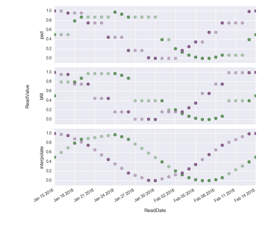
We can clearly see how in the top figure, the gaps have been filled with the last known value, in the middle figure, the gaps have been filled with the next value to come and in the bottom figure the difference has been interpolated.
Summary and Conclusion
In this post, we have seen how we can use PySpark to perform end-to-end interpolation of time series data. We have demonstrated,
how we can use resample time series data and how we can use the
Window function in combination with the first() and last()
function to fill-in the generated missing values. We have then seen, how we can use a user-defined function to perform a simple
spline-interpolation.
I hope this post helps to plug the gap of literature about end-to-end time series interpolation and does provide some usefulness for the readers.
Leave a Comment